Back to the Future: Solving the time-travel problem in machine learning

In Back to the Future II, Marty McFly gets an idea to purchase a sports almanac in the future and bring it back to the past to use for betting. Doc Brown warns him not to profit from time travel because information from the future could create dangerous effects and paradoxes in the past. But it’s too late: Marty’s nemesis, Biff, overhears the conversation, steals the time machine, and uses Marty’s plan to wreak havoc. As Marty learned the hard way, not properly respecting time can have dire consequences. And it turns out that when training machine learning models, we must also heed Doc’s warnings in order to avoid our own disasters.

Using machine learning models to predict the future is a powerful tool for creating or enhancing software applications. ML-driven predictions can power content recommendations, risk assessment, ads targeting, and much more. By understanding the probability of future outcomes, these machine learning applications deliver personalized experiences that benefit the user and the business.

In order to create a model that can predict future events, we train it on labeled examples from the past. For example, if we want to predict if a user will click on an ad, we need past examples of users clicking (and not clicking) on ads for the model to learn from. And it’s extremely important that when we construct this training data set, we make sure not to accidentally use information from the future in any one example. This problem is a form of data leakage and if handled incorrectly, it can have disastrous effects on model quality.

The data leakage conundrum

When a model makes a prediction about the future in real-time it is only capable of leveraging information up to the present moment. Without an almanac in hand or a DeLorean time machine, it is impossible to leverage anything beyond what we know about the world through our data right now. This makes data leakage from the future a non-issue when making real-time predictions. In fact, we typically want to use all available data to ensure the best predictions. Hence we just query our data sources for the latest known feature values and pass those to the model. So far so good, but this gets much more problematic when we rewind the clock to use past events for training our models.

When we construct our training data set of past events, we must be sure to only use feature values that were known prior to each event. It may seem natural to use the same query for fetching features that we use at prediction time, but this would fetch present-day values that weren’t available in the past.

The practical outcome of this would be models that seem to work great in offline validation tests, but act erratically in production. This is because the model got trained on information from the future that it won’t have during serving! It’s like taking away Biff’s sports almanac. Suddenly his predictions won’t be so great. Data leakage problems like this are not easy to catch and are hard to debug. They have plagued many data science teams and unfortunately are not simple to solve, especially in real-time use cases.

Getting accurate historical feature values

To avoid data leakage in model training, we need a dataset of historical feature values that represent the state of the world as of the time of events in the past. There are two ways we can go about generating these historical feature values.

The “log and wait” approach

One way to generate this data set is to start logging feature values as they’re fetched for the model in real time. For example, if we want to add the feature “ad_click_count_in_last_7d”, we can start calculating this in real time and logging it every time we show an ad. These features won’t be passed to the model because it hasn’t been trained with them yet, but they can be logged for future training jobs. We can later label this data to create a training data set with no leakage. The major advantage of this approach is that we are using the exact feature data from the time of the prediction event which can eliminate skew problems in many cases. This approach is used by many sizable machine learning organizations, but it also has a couple of drawbacks:

1. It takes time — If we want to create and test a new feature for a model, we need to build a pipeline for fetching the feature values, add it to the real-time prediction service, deploy it to production, and begin our logging. This could mean waiting weeks or months to have enough new feature data to create a training dataset. Meanwhile, older training datasets of historical events are obsolete because they do not contain the new feature.
2. The feature data becomes more difficult to use in other ML use cases that require the same feature. Because the logged data is specific to the prediction times and population distributions of the first use case it would typically require logging the feature data again for different use cases.

In some use cases where millions of predictions are made every day and seasonality is low, the “log and wait” approach isn’t so bad because collecting a large new training dataset may only take a day or two. However, for many machine learning applications, this is not the case.

Backfilling data and point-in-time joins

How do we get historical feature values without logging and waiting? If we don’t want to wait a year to have a year’s worth of training data for every new feature we create, maybe we can imagine what that feature value would have been if we were calculating it in the past. To do this, we can use the data we do have about past events (like log data) to reconstruct the feature value. This process is known as backfilling. For example, we could use historical click events on ads to calculate users’ click-through rates over seven day windows in the past.

Backfilling can be difficult as it requires efficiently reconstructing historical information. For example, we may have features with overlapping aggregation windows that become prohibitively expensive to compute across time without specialized optimizations. It is also critical that we are able to accurately represent historical data when backfilling. When training a model we want to minimize the error between the historical outcomes (the training data) and the predictions the model would have made at that time. Therefore any errors in backfilling could result in poor training data and lead to lower model accuracy. 

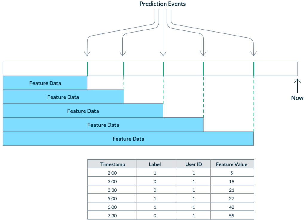
If we manage to accurately backfill historical values, we then need a way to select feature values from the right points in time for our training examples. With the “log and wait” approach, this is not necessary because the feature value times are implicitly logged with the time of the prediction event. However, when we construct training data with features that were generated independently of the prediction events, we have to choose the feature value cutoff time for each labeled event.

Snapshot-based time travel

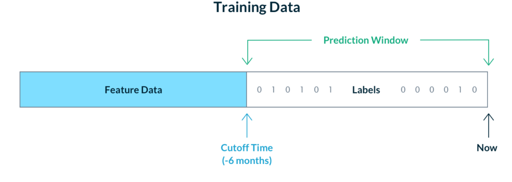
One simple solution to this problem is to choose a single cutoff time for all feature values. Technologies such as Delta Lake and Apache Hudi make it easy enough to fetch data from a single point in time. This approach makes some sense for models with slow-moving signals or large prediction windows. For example, a model predicting customer churn in the next 6 months may train on feature values up to t minus 6 months and labels from t minus 6 months until now. This approach is valid when feature data doesn’t change too frequently, although it is still limited compared to training across many different 6 month windows, each with different feature value cutoff times.

Continuous time travel

In cases where real-time information makes a meaningful difference, feature value cutoff times can vary for every single label! Examples include ad targeting or recommendation systems where user behavior is rapidly changing. In these real-time prediction use cases, we want to consider all possible feature data up until the time of the prediction event in order to be as accurate as possible. This means constructing a training dataset with thousands, or even millions of different cutoff times for each label. We call this process a “point-in-time join” and the logic to implement this is complex and brittle, so much so that many ML teams simply accept the “log and wait” approach.

Time-travel with Tecton

Lacking data infrastructure that’s designed with machine learning in mind, many teams struggle to solve the time-travel problem. However, it doesn’t need to be this hard. There are only two things that a data scientist should need to specify in order to easily construct high-quality training data sets:

1. The training events for which to fetch features
2. The list of desired features to fetch

That is exactly what Tecton enables. If a data scientist wants a set of features for a set of training events, then all they have to do is ask. Tecton does the heavy lifting of performing point-in-time joins to deliver the right values at the right time, so that modelers can focus on modeling and be confident that they’re getting high quality, accurate training data sets.

But what about adding new features? If a data scientist wants to create and test a new feature, they only need to provide Tecton with three things: the raw data source, the feature transformation in code, and the feature value calculation frequency. That’s it. From there, Tecton will backfill historical feature values and ensure the ongoing calculation and serving of features for both model training and predictions. In addition, Tecton makes these features available to be discovered and reused across your organization.

At Tecton we believe that making machine learning operational should be a simple and reliable process. While our models should carefully avoid using data from the future, our data platforms should feel like they are from the future. If you are interested in coming along for the ride, then sign up for early access! Where we’re going, we don’t need roads.